Bigger cities tend to be more productive and pay higher wages, but they also cost more to live in. In their BSE Working Paper (No. 804) “Optimal Spatial Taxation: Are Big Cities too Small?” Jan Eeckhout and Nezih Guner analyze how federal income taxes affect the size of cities by characterizing how optimal taxes reallocate workers across cities in the United States, and the implications for the overall economy.
Taxation and labor movement
Depending on how we tax someone we may end up distorting her decision. So when economists study taxation they tend to ask what choices would one have made if, perhaps, they were taxed differently. That is, would that person’s welfare (in a sense, their well-being) be different and possibly better? Since larger cities are more productive and pay higher wages, progressive federal tax policies in the US tax an equally skilled worker higher in larger cities than in smaller ones. While an identically skilled person earns 50% more in New York City than her “skill twin” in Asheville, North Carolina, she also pays on average almost 5% points more in taxes. Furthermore, housing is more expensive in New York City than it is in Asheville. Then a natural question is: would she be better off in New York City or Asheville?
Eeckhout and Guner pose that question more generally to the mobility of workers across labor markets. While higher wages will generally attract more workers, higher housing prices will deter them until equilibrium is reached. But taxation can play a hidden role in misallocating labor spatially by distorting choices. To pin down the role of taxation on labor mobility the authors engage general equilibrium techniques to evaluate the effect of taxes when accounting for how mobility will in turn change housing prices. Previous research looked at this question with partial equilibrium models, where one price is allowed to change but the others are assumed to remain constant. But such models have limited capacity of evaluating optimal tax policies or running experiments since the equilibrium effect of all price changes will determine the tax schedule and its implication. General equilibrium can do just that.
Two-city example
Before quantifying the spatial misallocation in the US, Eeckhout and Guner consider first a simple two-city model to generate insights. Imagine a world where all individuals are identical and decide whether to live in City 1 or City 2. City 2 is more productive and workers living there, independent of how many of them choose to live there, enjoy higher wages. Each city has a fixed amount of land used for housing. Since the land is limited in supply, as more people live in a city, housing prices goes up. In equilibrium individuals should be indifferent where to live. The land is owned partly by everyone living in the economy and partly by landlords who live elsewhere. The size of these absentee landlords captures the concentration of housing wealth in the economy.
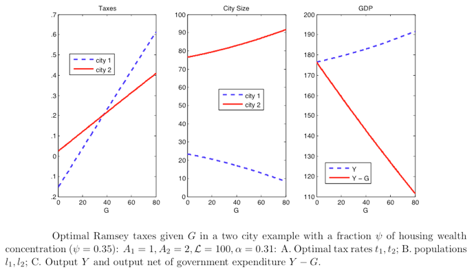
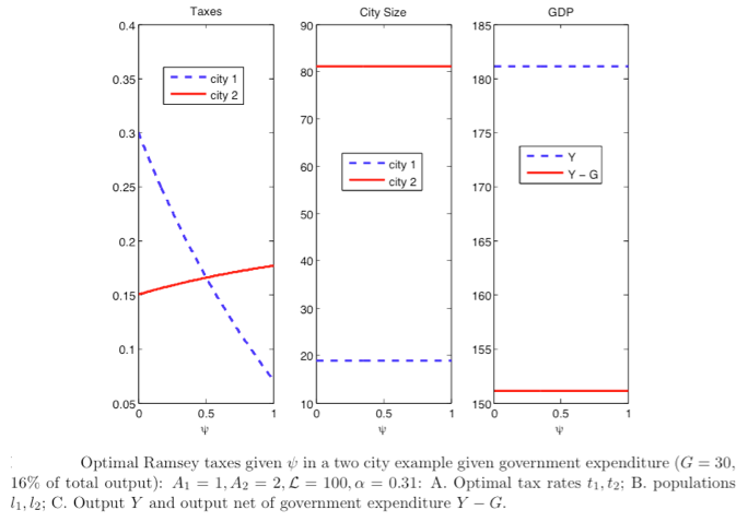
Imagine now a planner who has to raise a given level of revenue and can choose how much income taxes people living in City 1 and City 2 should pay. The planner chooses city-specific taxes to make individuals as better off as she can. The planner’s role is to determine taxes and then let individual decide optimally where to live and the equilibrium in the housing market to unfold. What would be the optimal level of taxes, and how the optimal taxes, city size and output (GDP) react to the size of government (i.e. how much revenue needs to be raised) and to the concentration of land ownership (i.e. who would benefit from a rise in housing prices)? Figures 1 and 2 below answer these questions.

Figure 1 shows what happens as the size of the government (G) increases. The most efficient way of raising a given level of revenue for the planner is to lower taxes in the more productive city. This will attract more workers there and increase the tax base. There is, however, a trade-off: as more people move to the more productive city, housing prices go up and workers start living in smaller and smaller houses. This lowers their welfare. As a result, when the government revenue needs are small, the planner prefers to have lower taxes in less productive city (and higher taxes in more productive one). As the revenue needs increase, however, the planner finds it optimal to have lower taxes in the more productive city (and relatively higher ones in less productive one). As shown in the first panel of Figure 1 above the tax in Big City 2 increases at a smaller rate than that of Small City 1 when government spending increases. This induces a population movement as shown in the second panel, with a divergence in the population distribution between the big and small city.

What about the concentration of housing wealth? When the size of absentee landlords (the parameter Ψ in Figure 2) is small, the planner finds it optimal to have low taxes in the more productive city (and high taxes in the less productive one). Lower taxes in more productive city attract more workers there and make it easier for the planner to collect a given level of revenue. The drawback is of course the higher housing prices that result from larger population in the more productive city. When the size of the absentee landlord is small, however, the whole population benefits from higher housing (land) prices. As the size of absentee landlords increase, however, the effect of higher housing prices started to have a bite, and as Figure 2 illustrates, taxes in the more productive city (city 2) increase and the ones in less productive city (city 1) decline. Because locating to the larger city raises housing prices in general, and the amount that goes to landlords, city size stays roughly constant. Further, output gains that would arise by having more people in the big, productive city disappear since the landlords are pocketing these gains.
What is the optimal tax and its implication on spatial misallocation of workers?
Drawing from US data and tax information from the OECD tax-benefit calculator, the authors first estimate the current progressivity and average level of federal taxes in the US. The estimated tax function generates the effective taxes paid on the average wage in each Metropolitan Statistical Area (MSA) across the US. Calibrating their model with these and other parameters drawn from the data, Eeckhout and Guner simulate the current US economy to establish their benchmark.
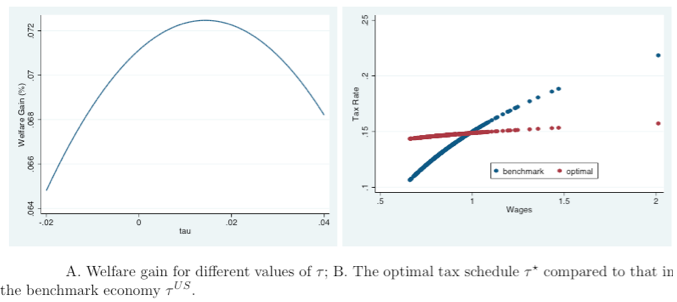
What the authors want to answer then is what allocations of workers would exist across the MSAs when tax schedules are such that welfare is maximized in the economy (relative to the benchmark). In particular, they find the optimal level of tax differences between less and more productive MSAs, while keeping the total tax revenue as it was in the benchmark economy. They find that the optimal tax is less progressive than what is currently estimated for the US. The tax schedules are presented in Figure 3 below and show that compared with the current US schedule bigger cities pay lower average taxes (those with average wages greater than 1 – wages of each MSA is normalized to the average wage across all MSAs).

The implications of implementing the optimal tax schedule and thus increasing the after-tax wages for those in larger cities is that workers migrate to the bigger, more productive cities. But this movement also raises housing prices. This forces people to substitute between their housing consumption (how big of a place they live in) and their consumption goods. So those in the larger cities end up living in smaller homes to be able to increase their consumption of other goods. This substitution is so nearly 1-to-1 that the welfare gain in the new economy is very small, at only a 0.0725% increase. The overall results for the economy can be seen below in Table 1.
[table caption=”Benchmark Economy, move from τ to τ*” width=”400″]
Outcomes[attr style=”text-align:left;”],
Welfare gain (%), 0.0725
Output gain (%), 1.57
Consumption (%), 1.53
Housing Consumption (%), -1.75
Population change top 5 cities (%), 7.95
Fraction of Population that Moves (%), 3.47
Change in average prices (%), 5.32
[/table]
The table illustrates that 3.5% of the population will migrate leading to a 5.3% average increase in housing prices and an overall increase of 1.6% in GDP. This masks the large population movements at the extremes, where the most productive city increases their population by 40% and the least productive city sees their population decline by 24%. Such is the scope of the spatial misallocation. Housing prices also experience large changes in the extremes where the top city sees a 23% increase while the least productive one experiences a nearly 9% decline (detailed in Table 1 in the authors’ paper).
Eeckhout and Guner further explore the sensitivity of their model to changing key inputs. Two of these, increasing government spending and the concentration of wealth, show results in line with what was concluded in the two-city planner problem. In all cases welfare gains remain small because potentially large output gains obtained by improving the tax schedule and reducing the spatial misallocation are offset by the housing prices that result from the migration. Moreover, optimal taxes in these settings are generally less progressive (or even regressive) than the current schedule of US taxes leading to higher output gains.
Should we tax bigger cities differently?
Fundamentally, what matters for population allocations across cities is the level of government spending and the concentration of housing wealth in the economy, since the optimal taxes that induce migrations are dependent on these factors. And because optimal taxes are generally less progressive than the current schedule, bigger cities are favored through population growth vis-à-vis lower average taxes. This will generate output growth in the wider economy but with a cost to workers living in these larger cities because of the increase in housing prices. Eeckhout and Guner rhetorically ask whether big cities are too small to make their point that perhaps big cities should be taxed differently than smaller ones, characterizing the effect of implementing such policies. They find that the gains in output outweigh the increased cost of living.


